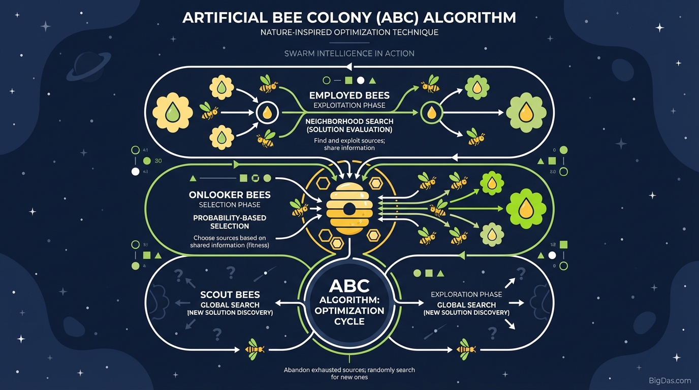
Artificial Bee Colony (ABC)
 Modern scientific illustration of Artificial Bee Colony (ABC)
A Practical Guide to Artificial Bee Colony (ABC) Optimization
Optimization problems often trap gradient-based solvers in local optima, where a solution looks correct in one region but misses a much better answer elsewhere. The Artificial Bee Colony (ABC) algorithm avoids this by using a population of agents that explore the search space stochastically, guided by rules borrowed from honey bee foraging.
ABC fits problems that are non-linear, non-differentiable, and high-dimensional: hyperparameter tuning, route planning, structural design, image segmentation. It needs no gradients, few parameters, and scales well with dimensionality.
What is Artificial Bee Colony (ABC)?
ABC is a metaheuristic optimization algorithm introduced by Karaboga in 2005. It models the foraging behavior of a honey bee swarm.
In the model:
- A food source is a candidate solution.
- Its nectar amount is the fitness (quality) of that solution.
- The colony is split into three bee types, each with a distinct role.
Employed Bees
Each employed bee is assigned to a specific food source. The bee evaluates the source, stores its position and nectar amount, and returns to the hive. Algorithmically, this is a local search: the bee generates a neighboring solution and uses greedy selection to keep the better of the two.
Onlooker Bees
Onlooker bees wait in the hive and pick a food source to exploit based on the probability reported by the employed bees. A source with higher nectar is chosen more often, so search effort concentrates on the most promising regions.
Scout Bees
When a food source cannot be improved after a fixed number of trials, the employed bee assigned to it abandons the source and becomes a scout. The scout generates a new, random solution within the search space. This is the mechanism that prevents the algorithm from stagnating in local optima.
Why Use ABC?
1. Strong Global Search
Many population-based algorithms converge prematurely to a local optimum. The scout phase keeps the population diverse by periodically replacing the worst, stagnant solutions with fresh random ones.
2. Few Parameters
ABC requires only the colony size and the abandonment limit. There is no inertia weight, no crossover rate, no mutation probability. This makes the algorithm easy to configure and tune.
3. Scales to High Dimensions
ABC handles problems with hundreds of variables. Because each candidate solution is evaluated independently and the variation step uses a single partner solution, the per-iteration cost grows linearly with dimension.
4. Memory of Past Solutions
Employed bees retain the best position found at their food source. The search uses past information, not just random samples.
How ABC Works: Step by Step
Step 1: Initialization
- Define the objective function $f(\mathbf{x})$ and the search bounds $\mathbf{x} \in [\mathbf{L}, \mathbf{U}]$.
- Set the population size $SN$ (equal to the number of employed bees).
- Set the Limit parameter, the number of failed trials before a source is abandoned.
- Initialize $SN$ food sources randomly within the bounds.
- Set the trial counter $trial_i = 0$ for each source.
Step 2: Employed Bee Phase
For each employed bee $i$, generate a new candidate solution:
$$v_{ij} = x_{ij} + \phi_{ij}(x_{ij} - x_{kj})$$
where:
- $k \neq i$ is a randomly chosen partner index,
- $j$ is a randomly chosen dimension,
- $\phi_{ij}$ is a uniform random number in $[-1, 1]$.
If $f(\mathbf{v}_i)$ is better than $f(\mathbf{x}_i)$, replace $\mathbf{x}_i$ with $\mathbf{v}_i$ and reset $trial_i = 0$. Otherwise, increment $trial_i$.
Step 3: Onlooker Bee Phase
Calculate the selection probability for each food source using fitness-proportional (Roulette Wheel) selection:
$$p_i = \frac{fit_i}{\sum_{n=1}^{SN} fit_n}$$
Onlooker bees choose a source according to $p_i$ and run the same local search and greedy selection as the employed bees.
Step 4: Scout Bee Phase
Find the source with the largest $trial_i$. If $trial_i > \text{Limit}$, replace $\mathbf{x}_i$ with a new random solution within the bounds and reset $trial_i = 0$.
Step 5: Termination
Repeat Steps 2 to 4 until the Maximum Cycle Number (MCN) is reached, a satisfactory fitness is achieved, or the convergence curve flattens. Output the best solution found.
Common Applications
1. Neural Network Training
ABC can train feed-forward networks by treating weights and biases as the search vector. It avoids the local minima that backpropagation sometimes gets stuck in.
2. Engineering Design
ABC handles non-linear, constrained problems such as truss weight minimization, aerodynamic shape design, and gear train design.
3. Image Processing
ABC is used for multi-level image thresholding. It finds the threshold values that maximize intra-class variance (Otsu's method) or minimize intra-class error in the image histogram.
4. Routing and Scheduling
ABC solves the Traveling Salesman Problem (TSP) and vehicle routing problems. Discrete and binary variants exist for these tasks.
Practical Tuning Advice
The single most important parameter is the Limit. A common default is:
$$\text{Limit} = SN \times D$$
where $D$ is the number of dimensions.
- Limit too low: Sources are abandoned too early, the algorithm behaves like random search, and good solutions never get refined.
- Limit too high: The algorithm clings to mediocre solutions and converges prematurely to a local optimum.
A reasonable starting configuration for most continuous problems is $SN = 50$, $\text{MCN} = 2000$, and $\text{Limit} = SN \times D$. Watch the convergence curve: if it flattens early, lower the Limit to encourage more scouting.
Frequently Asked Questions (FAQ)
1. How does ABC differ from Particle Swarm Optimization (PSO)?
PSO updates each particle's velocity using its own best position and the swarm's global best. ABC uses a division of labor and roulette-wheel selection instead. ABC typically explores more broadly, while PSO often converges faster but can get stuck in local optima.
2. Can ABC handle discrete problems?
Yes. Binary ABC (BABC) maps continuous values to ${0, 1}$ using a sigmoid transfer function, and discrete variants exist for integer, permutation, and combinatorial problems such as scheduling and the knapsack problem.
3. What is the "Limit" parameter?
The Limit is the number of consecutive failed trials allowed at a food source before the employed bee abandons it and becomes a scout. It controls the balance between local refinement and global exploration.
4. Is ABC computationally expensive?
Per iteration, ABC only evaluates the objective function and generates a new candidate via a single subtraction and addition. There is no gradient, no matrix factorization, and no expensive operator. It runs well on standard hardware and parallelizes trivially because each candidate solution is evaluated independently.
Summary
ABC solves non-linear, non-differentiable optimization problems using a population of agents modeled on honey bee foraging. Employed bees perform local search, onlooker bees allocate effort probabilistically, and scout bees maintain diversity by replacing stagnant solutions. The algorithm needs few parameters, scales to high dimensions, and applies to continuous, discrete, and combinatorial problems.