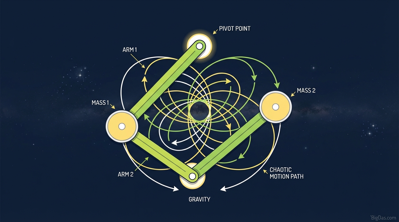
Double Pendulum
 Modern scientific illustration of Double Pendulum
Double Pendulum Simulation Tool
A simple pendulum is predictable: drop it, it swings back and forth at a regular rate. Attach a second pendulum to the end of the first, and the motion becomes chaotic. This is the double pendulum, and it is the most common textbook example of deterministic chaos in classical mechanics.
The following guide covers the physics behind the system and how to use the browser-based simulation tool to explore it.
What is a Double Pendulum?
Simple vs. Double Pendulum
A simple pendulum has a single bob on a rigid rod. Its motion is governed by the small-angle approximation of simple harmonic motion and is fully solvable.
A double pendulum adds a second rod and bob to the end of the first. The equations of motion are still derivable using Lagrangian mechanics, but they are nonlinear and coupled, which makes the long-term behavior highly sensitive to starting conditions.
Chaos and the Butterfly Effect
The double pendulum is the standard example used to teach Chaos Theory. A chaotic system is deterministic, meaning the laws of physics fix the outcome for a given initial state, but the equations are nonlinear enough that infinitesimal changes in the initial angle produce wildly different trajectories within seconds. This sensitivity is the Butterfly Effect: a change of 0.01° in the starting angle is invisible for the first few swings, then the two systems diverge completely.
The motion is not random, since conservation of energy and momentum strictly apply. The unpredictability comes from the nonlinearity, not from any randomness in the equations.
Features of the Tool
1. RK4 Integration
Most browser simulations use Euler integration, which leaks energy and causes the pendulum to drift unrealistically over time. This tool uses a 4th-order Runge-Kutta (RK4) integrator to keep the total mechanical energy stable.
2. Adjustable Parameters
Every physical parameter is exposed in the control panel:
- Masses: $m_1$ and $m_2$ for the top and bottom bobs.
- Lengths: $l_1$ and $l_2$ for the two rods.
- Gravity: Set to Earth's $9.81 \text{ m/s}^2$, the Moon's $1.62 \text{ m/s}^2$, or any custom value.
- Damping: A friction coefficient to simulate air resistance and bearing drag.
3. Motion Traces
Toggle a long-exposure trail behind the bobs. The path drawn by the lower bob forms spirograph-like fractals that are useful for studying the geometry of chaotic orbits.
4. Live Energy Plot
A side panel graphs Kinetic Energy ($T$), Potential Energy ($V$), and Total Energy ($E$) in real time. With damping set to zero, $E$ should remain constant; any visible slope means the integrator is leaking energy.
5. Time Dilation
A playback speed slider ranges from 10% to 100%. At low speeds, you can watch the exact moment the lower pendulum passes the unstable inverted equilibrium and tumbles into a full rotation.
How to Use the Tool
Step 1: Set the Initial Angles
When the page loads, the pendulum is paused. Click and drag either bob to set the starting angles $\theta_1$ and $\theta_2$. A good starting point for dramatic chaos is near the inverted position ($\theta_1 \approx \theta_2 \approx 180°$), which is an unstable equilibrium.
Step 2: Adjust the Parameters
Open the control panel and set the masses and lengths.
- For maximum chaos: Set $m_1 = m_2$ and $l_1 = l_2$. Symmetric configurations tend to produce the most energetic tumbling.
- For "whip" behavior: Set $m_1 \gg m_2$. The heavy top acts as a driver, and the light bottom whips around the joint.
Step 3: Enable the Trace
Before pressing play, turn on Trace Path and pick a high-contrast color against the background.
Step 4: Run the Simulation
Press Play. For the first few seconds, the motion may look regular. Once the lower bob gains enough kinetic energy to complete a full loop, the trajectory becomes unpredictable.
Step 5: Add Damping
After running a frictionless simulation, raise the damping slider. The chaotic flips will gradually transition to damped harmonic swinging, then to rest. This is a good way to watch energy dissipation in real time.
Use Cases
Physics Students and Educators
The Lagrangian for the double pendulum is $$L = T - V$$ where $$T = \frac{1}{2}(m_1 + m_2)l_1^2 \dot{\theta}_1^2 + \frac{1}{2}m_2 l_2^2 \dot{\theta}_2^2 + m_2 l_1 l_2 \dot{\theta}_1 \dot{\theta}_2 \cos(\theta_1 - \theta_2)$$ and $$V = -(m_1 + m_2)g l_1 \cos\theta_1 - m_2 g l_2 \cos\theta_2.$$ Applying the Euler-Lagrange equations to this $L$ gives the equations of motion, which the simulator solves numerically. The tool is useful for demonstrating:
- Conservation of energy.
- The qualitative difference between linear and nonlinear systems.
- Phase space and the divergence of nearby trajectories.
- How angular momentum transfers between coupled bodies.
Programmers
The double pendulum is a standard benchmark for testing physics engines. The tool can serve as a reference: if your own Python or C++ simulation drifts, gains energy, or "explodes," compare its behavior against the RK4 output here to debug the timestep or integrator choice.
Artists and Designers
The trace paths are deterministic generative art. The screen can be captured or exported for use in motion graphics, logo design, or as backgrounds for visual projects.
Experiments to Try
The Twin Test: Open the tool in two browser tabs side by side.
- In Tab A, set $\theta_1 = 90°$.
- In Tab B, set $\theta_1 = 90.01°$.
- Start both at the same time.
The two pendulums will look identical for the first 10 to 15 seconds, then diverge completely. This is the cleanest possible visual demonstration of sensitivity to initial conditions and is the reason long-term weather and turbulence prediction fails.
The Low Gravity Test: Set gravity to $1.62 \text{ m/s}^2$ (Moon). The lower bob completes more full rotations before energy is traded back to the upper rod, and the trace paths become more tightly wound.
Frequently Asked Questions (FAQ)
1. Is the motion of the double pendulum random?
No. It is deterministic. Given identical initial conditions with infinite precision, the path is reproducible. In practice, you cannot measure or input angles with infinite precision, so the long-term behavior is unpredictable. The chaos is in the equations, not in the data.
2. Can I achieve perpetual motion with this tool?
In the simulation, yes. Setting damping to 0% models a frictionless pivot in a vacuum. The total energy $E = T + V$ stays constant, and the pendulum swings forever. In any real apparatus, bearings and air resistance will dissipate energy.
3. Why does the pendulum sometimes spin in full loops?
When the lower bob reaches the top of its arc, it has maximum potential energy. As it falls, that converts to kinetic energy. Depending on the rod lengths and masses, the transfer of momentum from the upper rod can add to this kinetic energy, giving the lower bob enough speed to clear the inverted position and complete a full rotation. Small parameter changes dramatically alter how often this happens.
4. What is the Lagrangian, and why use it?
The Lagrangian $L = T - V$ is the difference between kinetic and potential energy. Applying the Euler-Lagrange equations, $$\frac{d}{dt}\left(\frac{\partial L}{\partial \dot{q}_i}\right) - \frac{\partial L}{\partial q_i} = 0$$ for each generalized coordinate $q_i$ produces the equations of motion. This approach is cleaner than resolving forces with $F = ma$, because the rod tensions (which are internal constraint forces) never need to be calculated directly.
Further Reading
The double pendulum is covered in most undergraduate classical mechanics textbooks, including Goldstein, Marion & Thornton, and Taylor. For the numerical side, any text on ordinary differential equations will derive the RK4 method used in this tool.