Fourier Series

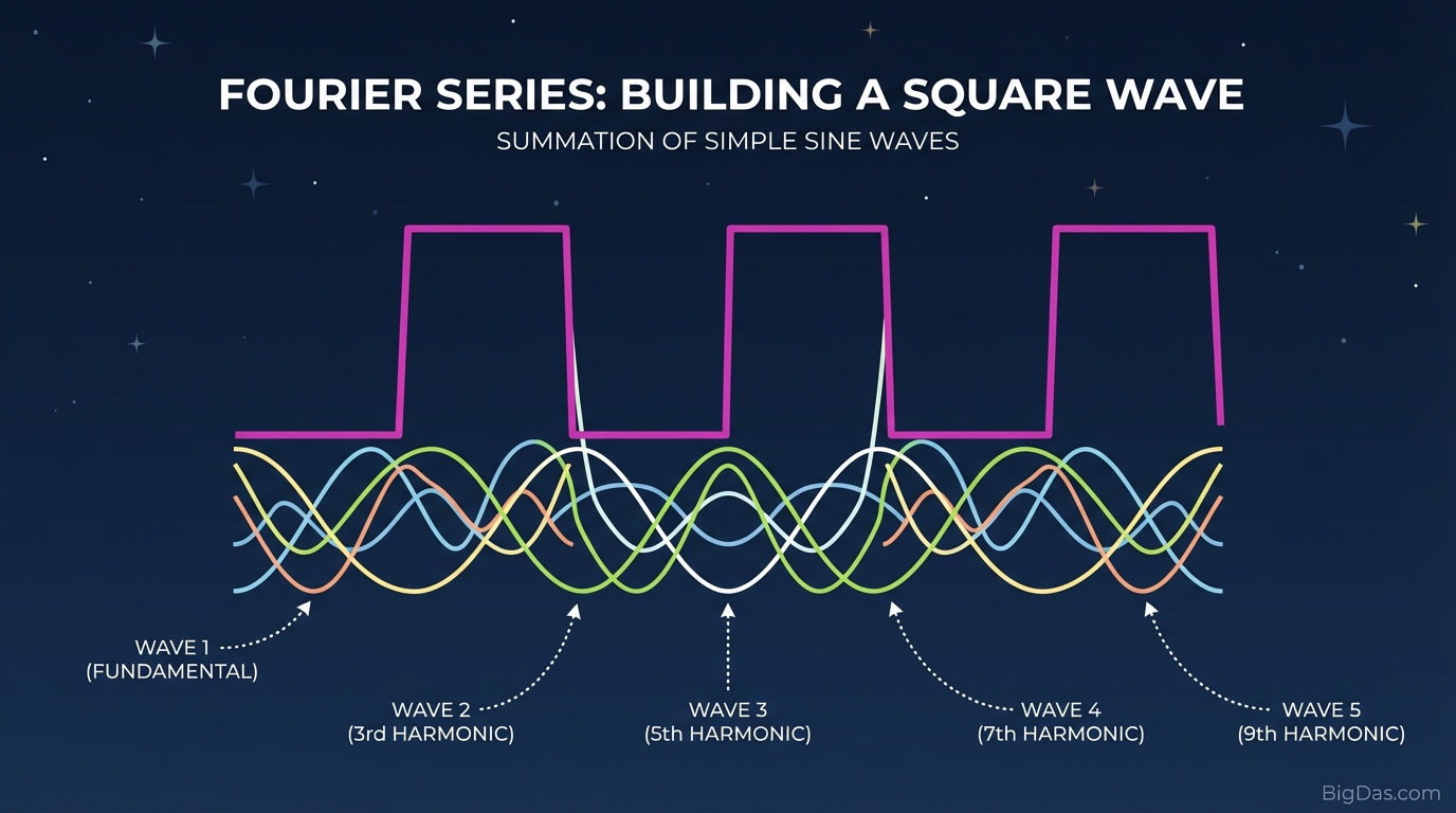
Visualize the Fourier Series and Square Wave Approximation
Staring at integrals and summation symbols ($\Sigma$) rarely builds intuition for the Fourier Series. The concept that a sharp, discontinuous square wave can be built from smooth, continuous sine waves is best understood visually, one term at a time.
This Interactive Fourier Series Visualization Tool lets you sum sine waves in real time to approximate a square wave, turning an abstract formula into a working model.
This guide covers what the Fourier Series is, why square wave approximation matters, and how to use the tool.
What is the Fourier Series?
The Fourier Series expresses a periodic function as a sum of sine and cosine waves. Joseph Fourier introduced this decomposition in the early 19th century to study heat conduction, and it has since become fundamental to signal processing, audio synthesis, and quantum mechanics.
The Square Wave
This tool focuses on the square wave. A perfect square wave switches instantly between 1 and -1. In the physical world, an instantaneous transition requires infinite energy. Mathematically, we approximate it by adding sine waves.
This process is additive synthesis. Start with a fundamental sine wave, then add odd harmonics at decreasing amplitudes:
$$f(x) = \sin(x) + \frac{1}{3}\sin(3x) + \frac{1}{5}\sin(5x) + \dots$$
What each term contributes:
- Fundamental frequency: sets the width of the pulse.
- 3rd harmonic: flattens the top of the wave.
- 5th, 7th, 9th harmonics: sharpen the vertical edges and flatten the plateau.
As terms accumulate, the wiggly sum converges toward a square block.
Key Features
1. Real-Time Rendering
Static images show the result. This tool shows the process. The rendering engine updates instantly as you add harmonics, so you can see how each new sine wave changes the sum.
2. Component Isolation
The display shows each individual sine wave alongside the running total. You can watch constructive and destructive interference combine into the final shape.
3. Scalable Iteration Count
Run the sum with 3 terms or 100 terms. Higher counts make the Gibbs Phenomenon (the overshoot spikes at the corners) clearly visible.
4. No Code Required
The interface runs in the browser. No MATLAB, no Python, no setup. Open the page and start adjusting parameters.
Step-by-Step Usage
Step 1: Start with the Fundamental (N=1)
Reset to the lowest setting. You will see a single sine wave rising and falling smoothly. This represents the pitch of the target square wave.
Step 2: Add the Third Harmonic (N=3)
Increase the iteration count. The 3rd harmonic (3× the frequency, 1/3 the amplitude) subtracts from the peak of the fundamental, beginning to flatten the top.
Step 3: Increase to N=5 and N=7
Add the next two odd harmonics. The rising and falling edges become steeper. The wiggles on top become smaller and faster. This is approximation in action: trading one large error for many small, high-frequency errors.
Step 4: Push to N=50+
From a distance, the wave looks like a clean square. Up close, sharp spikes protrude at every corner. This is the Gibbs Phenomenon, the mathematical fact that no finite sum of continuous functions can perfectly describe a discontinuous jump.
Use Cases
Electrical Engineers
Square waves drive clock signals in digital circuits. If a circuit acts as a low-pass filter and cuts high frequencies, the clean square becomes a rounded sine, and timing fails. This tool shows why bandwidth matters for digital signals.
Audio Engineers
A subtractive synth filters a square wave to shape its tone. An additive synth (like a Hammond organ) stacks sine waves to build sound from scratch. The tool demonstrates how harmonic content changes the timbre from a pure tone to a buzzy square.
Math and Physics Students
Teachers can use the tool to demonstrate limits and series convergence without writing equations at the board. The convergence becomes visible.
Data Scientists
The Fast Fourier Transform (FFT) decomposes signals into frequencies and powers JPEG, MP3, and active noise cancellation. The Fourier Series is the conceptual foundation.
Pro-Tips
- Predict the next ripple. Before adding a harmonic, guess where the new wiggle will appear. Higher harmonics oscillate faster.
- Watch the rising edge. The slope of the vertical edge gets steeper with more terms, but never truly vertical. Finite sums cannot produce an infinite slope.
- Track the energy distribution. Higher harmonics have very low amplitude, meaning most of the signal's energy lives in the lower frequencies. The sharpness of the corners comes from the high frequencies, not the bulk of the energy.
Frequently Asked Questions (FAQ)
1. Why only odd harmonics for a square wave?
A square wave has half-wave symmetry. Even harmonics (2×, 4×, 6×) break that symmetry and produce a lopsided wave, closer to a sawtooth. Only odd harmonics (1, 3, 5, 7…) preserve the required symmetry.
2. Will the sum ever become a perfect square?
In the limit of infinitely many terms, yes. In any finite sum, small ripples and Gibbs overshoot remain.
3. What is the Gibbs Phenomenon?
Spikes at the corners that persist no matter how many terms you add. The overshoot is roughly 9% of the jump and is unavoidable when a Fourier series approximates a discontinuity.
4. Can the tool visualize other waveforms?
This instance targets square waves to highlight the contrast between smooth sines and sharp edges. The same Fourier principle applies to triangle waves, sawtooth waves, and any periodic signal.
Conclusion
The Fourier Series shows that a discontinuous, sharp-edged signal is equivalent to a sum of smooth, continuous waves. Whether you are debugging a clock signal, designing a synth patch, or working through a calculus problem, watching the sum converge is the fastest way to build a working understanding of the result.