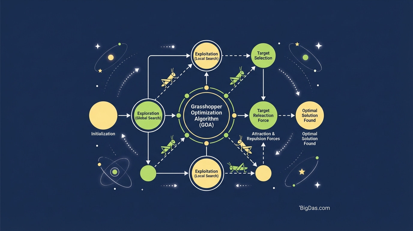
Grasshopper Optimization Algorithm (GOA)
 Modern scientific illustration of Grasshopper Optimization Algorithm (GOA)
Mastering the Grasshopper Optimization Algorithm (GOA): A Practical Guide
Finding a global optimum remains difficult for many engineering and machine learning problems. Gradient-based methods and classical heuristics get trapped in local optima, especially when the search space is non-linear, constrained, or high-dimensional.
The Grasshopper Optimization Algorithm (GOA) is a population-based meta-heuristic that simulates grasshopper swarming behavior. It models social forces between agents to balance exploration (global search) and exploitation (local refinement).
This guide covers the GOA model, its core equations, implementation steps, and practical applications.
What is GOA?
GOA is a nature-inspired meta-heuristic introduced by Saremi, Mirjalili, and Lewis (2017). It treats candidate solutions as grasshoppers in a swarm. Each grasshopper moves according to social interaction forces, gravity, and wind advection.
Biological Inspiration
Grasshoppers have two main life-cycle phases:
- Nymph phase: Slow movement with small steps (local search).
- Adulthood phase: Long-range, abrupt movement (global search).
GOA models both phases to maintain diversity early in the run and convergence near the end.
Exploration vs. Exploitation
- Exploration: The swarm covers a wide region of the search space.
- Exploitation: The swarm refines solutions near the best candidate found.
The adaptive parameter c gradually shrinks the comfort zone, shifting behavior from exploration to exploitation.
Social Forces
Each grasshopper experiences:
- Repulsion at short range (prevents premature clustering).
- Attraction at medium range (pulls agents toward promising regions).
- Comfort zone (the distance range where social interaction dominates).
This is the core mechanism that makes GOA different from PSO and GA.
Mathematical Model
The position update for grasshopper $i$ in dimension $d$ is:
$$X_i^d = c \left( \sum_{j=1, j \neq i}^{N} c \frac{ub_d - lb_d}{2} s\left(|x_i^d - x_j^d|\right) \frac{x_j^d - x_i^d}{d_{ij}} \right) + T_d$$
Where:
- $X_i^d$ is the position of grasshopper $i$ in dimension $d$.
- $ub_d, lb_d$ are the upper and lower bounds in dimension $d$.
- $T_d$ is the target (best solution) in dimension $d$.
- $c$ is a decreasing coefficient controlling the comfort zone.
- $s(r)$ is the social force function defining repulsion and attraction.
Social Force Function
The $s$ function is defined piecewise:
$$s(r) = fe^{-\frac{r}{l}} - e^{-r}$$
Typical values are $f = 0.5$ and $l = 1.5$. The function is positive (repulsion) for $r < 2.079$ and negative (attraction) between $r \approx 2.079$ and roughly 4, after which its effect becomes negligible.
Adaptive Parameter c
The coefficient $c$ decreases linearly with iterations:
$$c = c_{\max} - l \cdot \frac{c_{\max} - c_{\min}}{L}$$
Where:
- $c_{\max} = 1$ and $c_{\min} = 0.00001$ in most implementations.
- $l$ is the current iteration.
- $L$ is the maximum number of iterations.
This shrinking of $c$ gradually reduces the contribution of social forces, so the swarm converges toward $T_d$.
Key Features of GOA
1. Adaptive Comfort Zone
The linear decrease of $c$ automatically transitions the algorithm from exploration to exploitation. No manual scheduling is required.
2. Few Internal Parameters
The main tunable parameters are population size, maximum iterations, $f$, and $l$ in the $s$ function. Defaults work well for most problems.
3. Scalability
GOA handles both low-dimensional and high-dimensional problems. Population diversity is maintained through repulsion in early iterations.
4. Escape from Local Optima
Repulsion in early iterations prevents the swarm from collapsing onto a single point, reducing the chance of premature convergence.
5. O(N²) Cost per Iteration
Distance computation is pairwise, so cost grows quadratically with population. For $N \leq 100$ this is acceptable on modern hardware.
Step-by-Step Implementation
The workflow below applies to Python, MATLAB, or C++.
Step 1: Define the Objective Function
Specify:
- Inputs: Decision variables and their ranges.
- Constraints: Bounds and any penalty terms.
- Goal: Minimize or maximize.
Step 2: Initialize the Population
- Population size: 20 to 50 for most problems.
- Randomly sample positions within bounds.
- Evaluate fitness for each grasshopper.
- Set the best grasshopper as the Target $T$.
Step 3: Optimization Loop
For each iteration $l$ up to $L$:
- Update $c$ using the linear schedule above.
- Normalize distances in each dimension by $\frac{ub_d - lb_d}{2}$.
- Compute social forces using the $s$ function.
- Update positions with the position equation.
- Apply boundary checks (clamp to $[lb, ub]$ or reflect).
- Re-evaluate fitness and update $T$ if a better solution appears.
Step 4: Termination
Stop after $L$ iterations. The Target $T$ is the best solution found.
Practical Tip
Normalize all variables to a similar range (e.g. $[0, 1]$) before running GOA. This keeps the social forces balanced across dimensions and improves stability.
Common Variants
| Variant | Purpose | Key Modification |
|---|---|---|
| MOGOA | Multi-objective optimization | Archive of non-dominated solutions and roulette-wheel leader selection |
| BGOA | Binary problems (e.g. feature selection) | Sigmoid or transfer function converts continuous position to 0/1 |
| IGOA | Improved convergence | Modified $s$ function and non-linear $c$ schedule |
| HHO-GOA | Hybrid search | Combines Harris Hawks exploration with GOA exploitation |
Real-World Applications
Structural Engineering
Truss and frame weight minimization under stress and deflection constraints. GOA handles non-linear constraint penalties effectively.
Machine Learning
- Feature selection: BGOA selects subsets that maximize accuracy and minimize feature count.
- Hyperparameter tuning: GOA optimizes learning rate, regularization, and architecture parameters.
- Neural network training: Replaces or augments gradient descent to escape local minima in MLP weight space.
Control Systems
PID tuning, robotic trajectory optimization, and energy management in industrial processes.
Power Systems
Optimal power flow, unit commitment, and renewable integration planning.
Frequently Asked Questions
Q1: How does GOA differ from PSO?
PSO updates position using a velocity vector based on personal best and global best. GOA uses social forces (attraction and repulsion) between all pairs of agents. GOA's repulsion term reduces premature convergence, while PSO often converges quickly to the global best.
Q2: Can GOA handle multi-objective problems?
Yes. MOGOA maintains an archive of non-dominated solutions and uses a roulette-wheel mechanism to select leaders from sparsely populated Pareto regions.
Q3: What is the computational complexity?
Each iteration costs $O(N^2)$ due to pairwise distance calculations. For $N \leq 100$, runtimes are typically seconds to a few minutes.
Q4: Is GOA suitable for discrete problems?
The standard GOA targets continuous problems. For discrete or binary problems, use BGOA, which maps continuous positions to ${0, 1}$ via a transfer function (e.g. sigmoid or V-shaped).
Q5: What population size should I use?
Start with 20 to 50. Larger populations improve diversity but increase cost quadratically. For high-dimensional problems ($D > 100$), consider 50 to 100.
Q6: How sensitive is GOA to parameter choice?
Moderately. The $s$ function parameters ($f = 0.5$, $l = 1.5$) and $c_{\max}/c_{\min}$ defaults are robust across most benchmarks. Problem-specific tuning rarely changes results significantly.
Summary
GOA provides a straightforward implementation, requires few parameters, and balances exploration with exploitation through an adaptive comfort zone. It is well suited for continuous optimization tasks where gradient information is unavailable, expensive, or unreliable. For discrete, multi-objective, or large-scale problems, the MOGOA, BGOA, or hybrid variants extend the base algorithm effectively.