Grey Wolf Optimizer (GWO)
 Modern scientific illustration of Grey Wolf Optimizer (GWO)
Mastering the Grey Wolf Optimizer (GWO)
Many optimization problems are non-linear and high-dimensional. Traditional algorithms frequently get stuck in local optima and fail to locate the global minimum or maximum.
The Grey Wolf Optimizer (GWO) is a population-based meta-heuristic introduced by Mirjalili et al. in 2014. It models the social hierarchy and cooperative hunting behavior of grey wolves to search the solution space. Because it does not rely on gradient information, it works on problems that are non-differentiable, noisy, or discontinuous.
This guide covers the algorithm, the underlying math, and how to configure the GWO tool for your own problem.
What is the Grey Wolf Optimizer (GWO)?
GWO is a swarm intelligence algorithm. A swarm of candidate solutions, called "wolves," moves through the search space and converges toward the best-known position. The algorithm is derivative-free, requires only a few control parameters, and scales well to large search spaces.
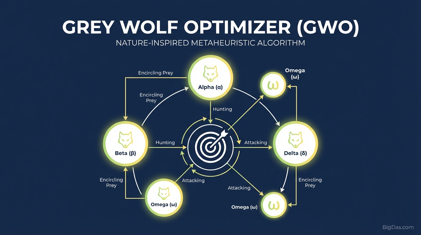
The social structure of a real wolf pack is mapped directly to the search process.
The Social Hierarchy of the Pack
Every candidate solution in GWO is treated as a wolf. Wolves are ranked by fitness at every iteration.
- Alpha ($\alpha$): The leader. Represents the best solution found so far. The entire pack updates its position relative to the Alpha.
- Beta ($\beta$): The second-best solution. Reinforces the Alpha and provides a secondary reference point.
- Delta ($\delta$): The third-best solution. Acts as a scout for better regions of the search space.
- Omega ($\omega$): All remaining candidate solutions. Each Omega updates its position based on the combined guidance of $\alpha$, $\beta$, and $\delta$.
The hunting (optimization) process is driven by the three leaders. The Omegas follow $\alpha$, $\beta$, and $\delta$ to converge on the global optimum.
Key Features
1. Balance of Exploration and Exploitation
Exploration searches new regions of the space; exploitation refines the search around the best-known solution. GWO controls this balance with the parameter $\vec{a}$, which decreases linearly from 2 to 0 over the course of a run. Early iterations favor exploration; later iterations favor exploitation.
2. Few Control Parameters
GWO requires only the population size, the maximum number of iterations, and the search bounds. There are no mutation rates, crossover probabilities, or inertia weights to tune.
3. Derivative-Free
The objective function is treated as a black box. GWO does not compute gradients, so it works on discontinuous, noisy, or time-varying problems.
4. Hierarchical Update Mechanism
Each Omega's new position is computed from the average influence of $\alpha$, $\beta$, and $\delta$. This structure reduces premature convergence relative to single-leader methods.
How It Works: The Hunting Phases
Phase 1: Initialization
A population of wolves is placed at random positions within the bounds of the search space. Fitness is evaluated for every wolf. The top three are assigned to $\alpha$, $\beta$, and $\delta$.
Phase 2: Encircling the Prey
Wolves update their position by encircling the leaders. The distance between a wolf and a leader is modeled by:
$$D = |\vec{C} \cdot \vec{X}_p(t) - \vec{X}(t)|$$
$$\vec{X}(t+1) = \vec{X}_p(t) - \vec{A} \cdot D$$
where $\vec{X}_p(t)$ is the position of the prey (leader) and $\vec{X}(t)$ is the wolf's current position. The coefficient vectors are:
$$\vec{A} = 2\vec{a} \cdot \vec{r}_1 - \vec{a}$$
$$\vec{C} = 2 \cdot \vec{r}_2$$
$\vec{r}_1$ and $\vec{r}_2$ are random vectors in $[0, 1]$. $\vec{a}$ decreases linearly from 2 to 0.
When $|\vec{A}| > 1$, wolves diverge from the leader, forcing exploration. When $|\vec{A}| < 1$, wolves converge toward the leader, forcing exploitation.
Phase 3: Attacking the Prey
The final position of each wolf is the average of the three best positions:
$$\vec{X}(t+1) = \frac{\vec{X}_1 + \vec{X}_2 + \vec{X}_3}{3}$$
where $\vec{X}_1$, $\vec{X}_2$, and $\vec{X}_3$ are the candidate positions computed from $\alpha$, $\beta$, and $\delta$ respectively. As $\vec{a}$ approaches 0, the pack converges on the prey.
Step-by-Step Guide: Using the GWO Tool
Step 1: Define Your Objective Function
Write the function you want to minimize or maximize. Example for a simple sphere function:
$$f(x) = x^2$$
Step 2: Configure the Population and Iterations
- Number of Wolves: 30 to 50 is a common starting range. Larger populations explore more but cost more per iteration.
- Max Iterations: 500 to 1000 is usually enough for non-trivial problems.
Step 3: Set Boundaries
Set the Lower Bound (lb) and Upper Bound (ub) for each variable. For a real engineering problem, the bounds reflect physical limits (e.g., beam thickness cannot be negative).
Step 4: Run the Optimization
At each iteration, the tool:
- Evaluates the fitness of every wolf.
- Updates $\alpha$, $\beta$, and $\delta$ to the three best positions.
- Updates every Omega based on the three leaders using the encircling and averaging equations above.
- Decreases $\vec{a}$ by one step.
Step 5: Analyze the Results
The tool outputs the Best Score (fitness of the Alpha) and the Best Position (variable values of the Alpha). These are the solution to your problem.
Common Use Cases
1. Engineering Design
GWO is used on benchmark problems such as the tension/compression spring design and the welded beam design, where the goal is to minimize weight or cost subject to stress and deflection constraints.
2. Machine Learning
GWO is used as a wrapper for feature selection and for tuning hyperparameters of Support Vector Machines and Neural Networks.
3. Power Systems
GWO solves the Economic Load Dispatch (ELD) problem, distributing generator output to minimize fuel cost while meeting demand and satisfying generator limits.
4. Path Planning
GWO finds collision-free paths for mobile robots by treating obstacles as repellents and the goal as the prey.
Practical Advice
- Hybridize for hard problems: For multi-modal landscapes, combine GWO with Genetic Algorithms or Differential Evolution to escape stagnation in later iterations.
- Use a custom decay for $\vec{a}$: A non-linear decay schedule can keep the pack more reactive when the optimum shifts over time.
- Add a penalty function: GWO is unconstrained by design. If a wolf leaves the feasible region, apply a penalty to its fitness so the Alpha never points the pack toward an invalid solution.
- Run multiple trials: GWO is stochastic. Average the results over 20 to 50 independent runs to assess reliability.
Frequently Asked Questions (FAQ)
1. How is GWO different from Particle Swarm Optimization (PSO)?
PSO updates each particle using its personal best and the global best. GWO updates each wolf using the three best solutions in the population. GWO's three-leader structure is generally more robust on multi-modal problems.
2. Is the Grey Wolf Optimizer deterministic?
No. GWO is stochastic because of the random coefficients $\vec{r}_1$ and $\vec{r}_2$ in the update equations. Independent runs may take different paths but should converge to similar results.
3. Can GWO handle multi-objective problems?
Yes. The Multi-Objective Grey Wolf Optimizer (MOGWO) extends GWO with an archive that stores non-dominated Pareto-optimal solutions, allowing it to approximate the Pareto front for problems with conflicting objectives.
4. What programming languages support GWO?
The algorithm is language-agnostic. Reference implementations are widely available in Python, MATLAB, C++, and Java. Python is the most common choice for data science applications.