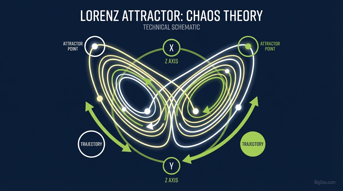
Lorenz Attractor
 Modern scientific illustration of Lorenz Attractor
Lorenz Attractor Visualization Tool
In 1961, meteorologist Edward Lorenz entered numbers into a computer to model weather patterns. He rounded a decimal from .506127 to .506, assuming the difference was trivial. The output was a completely different forecast.
That accident led to Chaos Theory and the Butterfly Effect, the idea that small changes in initial conditions can produce wildly different outcomes.
This page covers the math behind the Lorenz Attractor and how to use the visualization tool to explore deterministic chaos.
What is the Lorenz Attractor?
The Lorenz Attractor is the solution to a system of three ordinary differential equations. Edward Lorenz derived it by simplifying the Navier-Stokes equations to model atmospheric convection, how air moves as it heats and cools.
The Equations
The Lorenz system is defined by:
- $\frac{dx}{dt} = \sigma(y - x)$
- $\frac{dy}{dt} = x(\rho - z) - y$
- $\frac{dz}{dt} = xy - \beta z$
Variable definitions:
- x, y, z: Spatial coordinates of a point in the system.
- t: Time.
- $\sigma$ (Sigma): The Prandtl number (ratio of fluid viscosity to thermal conductivity).
- $\rho$ (Rho): The Rayleigh number (temperature difference between the top and bottom of the atmospheric layer).
- $\beta$ (Beta): A geometric factor describing the dimensions of the physical layer.
The Strange Attractor
When you solve these equations over time, the trajectory of (x, y, z) never intersects itself and never repeats. It orbits two points in a shape resembling butterfly wings. This fractal structure is a Strange Attractor.
The system is deterministic (governed by fixed rules) but chaotic (long-term behavior is unpredictable because tiny changes in the starting position produce entirely different paths).
Tool Features
1. Real-Time WebGL Rendering
The tool uses WebGL acceleration to render high-resolution trajectories in real time, keeping animations smooth even over long durations.
2. Full Parameter Control
The default Lorenz values are $\sigma=10$, $\rho=28$, $\beta=8/3$. The sliders let you change these values. Drop $\rho$ below 10 and the system spirals into a fixed point. Push $\rho$ above 90 and the orbits become more complex.
3. Multi-Trajectory Comparison
Spawn multiple particles with slightly different starting coordinates (e.g. 0.001 apart). They track together at first, then diverge, a direct visual of the Butterfly Effect.
4. 3D Phase Space Rotation
Zoom, pan, and rotate the model 360 degrees to see the depth of the wings and how trajectories weave through phase space.
5. Aesthetic Customization
Adjust trail colors, background themes, and line thickness. Export for presentations, digital art, or analysis.
How to Use the Tool
Step 1: Set Initial Conditions
The control panel has inputs for Starting Coordinates (x₀, y₀, z₀).
- Recommended: x=0.1, y=0, z=0.
- Click Initialize to place the point.
Step 2: Configure System Parameters
Sliders control Sigma ($\sigma$), Rho ($\rho$), and Beta ($\beta$).
- Standard Chaos: $\sigma=10$, $\rho=28$, $\beta=2.667$.
- Stable Orbit: Lower $\rho$ below 10, the system spirals into a fixed point.
- High Complexity: Increase $\rho$ to 90+ for wider orbits.
Step 3: Animation Controls
- Time Step (dt): Lower values (e.g. 0.01) give smoother curves but render slower. Higher values (0.05) are faster but less precise.
- Speed: Controls playback rate.
- Press Play to start the simulation.
Step 4: Test Divergence
- Pause the simulation.
- Select Add Shadow Particle to add a second point at x+0.0001.
- Resume and watch the two lines overlap, then separate to opposite sides of the graph.
Step 5: Export
- Snapshot downloads a high-resolution PNG.
- Export Data outputs CSV coordinates for external analysis.
Use Cases
Educators and Students
Demonstrate sensitivity to initial conditions in class. It makes differential equations tangible.
Data Scientists and Mathematicians
Verify Runge-Kutta integration methods or study phase space topology. Useful as a rapid-prototyping environment before building models in Python or MATLAB.
Artists and Designers
Generate organic curves for backgrounds, UI elements, or generative art prints. High-res exports make it useful for design assets.
Programmers
Examine how the tool handles timestep (dt) versus rendering speed for lessons on simulation loops and numerical stability.
FAQ
1. Why does the graph look like a butterfly?
The wings correspond to the two unstable equilibrium points. The trajectory spirals around one wing, gets repelled, then flips to the other. It oscillates unpredictably between them.
2. Is the pattern random?
No. It is deterministic. Identical inputs produce identical paths. But since physical measurements can't be infinitely precise, real-world chaotic systems appear random.
3. What happens if I change Rho to a very high number?
The system stays chaotic but the shape changes. Wings may merge or blur, and the trajectory moves faster between the two lobes.
4. Can this tool predict the weather?
Not directly. This is a simplified model. But it shows why long-term weather prediction (beyond ~10 days) fails: small data-collection errors compound over time.
Summary
The Lorenz Attractor is one of the most significant mathematical discoveries of the 20th century. It demonstrated that natural systems aren't linear and that predictability has hard limits.
The visualization tool lets you manipulate the constants that define the system and observe the results directly.
Start the simulator below to see the Butterfly Effect in action.
Launch the Simulator
Runs in your browser. No installation required.