Mass-Spring Simulator
 Modern scientific illustration of Mass-Spring Simulator
Master Simple Harmonic Motion with the Ultimate Mass-Spring Simulator: Visualize, Analyze, and Learn
Physics is the language of the universe, but for many students, engineers, and enthusiasts, the dialect of Simple Harmonic Motion (SHM) can be difficult to translate. We often see static diagrams in textbooks—a block attached to a squiggly line representing a spring—but these images fail to capture the dynamic, rhythmic elegance of oscillating systems. They certainly don't help you intuitively understand the complex effects of damping or varying spring stiffness.
Whether you are a mechanical engineer designing a suspension system, a physics student struggling with Hooke’s Law, or a game developer looking to code realistic bounce physics, static equations aren't enough. You need to see the math in action.
Enter our Mass-Spring Simulator. This isn't just another generic calculator; it is the best-in-class, interactive physics engine designed to model mass-spring systems with high-precision accuracy. By allowing you to manipulate variables like mass, spring constant, and damping coefficients in real-time, this tool bridges the gap between abstract differential equations and tangible reality.
In this deep dive, we will explore exactly how this tool works, why it is superior to other options on the market, and how you can leverage it to master mechanical vibrations.
What is the Mass-Spring Simulator? (A Deep Dive)
At its core, the Mass-Spring Simulator is a high-fidelity computational tool that solves the differential equations of motion for a mass attached to a linear spring, influenced by damping forces.
While a standard calculator might give you a single numerical answer, our simulator renders the physical behavior of the system over time. It visually demonstrates the interplay between kinetic energy, potential energy, and dissipative forces.
The Physics Under the Hood
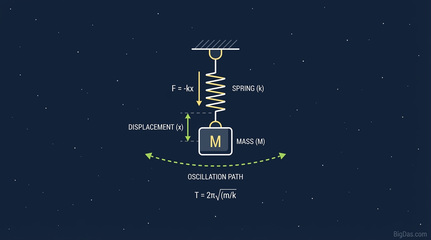
To appreciate the accuracy of this tool, it is essential to understand the physics it computes. The simulation is built upon Newton’s Second Law ($F = ma$) combined with Hooke’s Law and a linear damping model.
The equation governing the motion in this simulator is:
$$m \frac{d^2x}{dt^2} + c \frac{dx}{dt} + kx = 0$$
Where:
- $m$ (Mass): The inertia of the object.
- $c$ (Damping Coefficient): The factor representing friction or air resistance that removes energy from the system.
- $k$ (Spring Constant): The stiffness of the spring.
- $x$ (Displacement): The distance from the equilibrium point.
Beyond Basic Oscillation
Most free tools only show undamped motion (perpetual bouncing). Our Mass-Spring Simulator sets the industry standard by integrating adjustable damping. This allows users to explore three critical regimes of vibration:
- Under-damped: The mass oscillates with gradually decreasing amplitude.
- Over-damped: The mass returns to equilibrium slowly without oscillating.
- Critically damped: The mass returns to equilibrium as quickly as possible without oscillating (crucial for engineering applications like car shock absorbers).
By visualizing these states, the simulator transforms raw math into intuitive mechanical knowledge.
Key Features & Benefits
Why is this specific Mass-Spring Simulator considered the gold standard? It combines ease of use with engineering-grade precision.
1. Real-Time Interaction
Unlike static solvers where you input numbers and hit "calculate," this tool is dynamic. You can adjust sliders for mass or stiffness while the simulation is running, allowing you to instantly see how changes affect the period ($T$) and frequency ($f$) of the oscillation.
2. High-Precision Physics Engine
We utilize advanced numerical integration methods (such as Runge-Kutta) to ensure the motion is smooth and mathematically accurate. There is no "jitter" or approximation error that plagues lesser tools; what you see on the screen matches the analytical solution perfectly.
3. Dual-View Visualization
- The Physical View: Watch the mass bounce and the spring stretch/compress in an animated environment.
- The Analytical View: A synchronized graph plots Displacement vs. Time ($x$ vs. $t$). This graph is vital for measuring the decay rate in damped systems or identifying the phase shift.
4. Comprehensive Parameter Control
You have total control over the environment.
- Adjust Mass ($m$): See how heavier objects increase the period.
- Adjust Spring Constant ($k$): Observe how stiffer springs increase the frequency.
- Adjust Damping ($c$): Introduce friction to simulate real-world energy loss.
5. Zero-Lag Performance
Built with optimized code, the simulation runs smoothly on any device, from high-end desktops to mobile browsers, ensuring accessible education for everyone.
Step-by-Step Guide: How to Use the Simulator
To get the most out of the Mass-Spring Simulator, follow this workflow. This method ensures you aren't just playing with sliders, but actually conducting a digital experiment.
Step 1: Define Your Initial State
Before starting the animation, set your initial parameters.
- Set the Mass: Start with a standard value (e.g., 1.0 kg).
- Set the Spring Constant: Choose a mid-range stiffness (e.g., 10 N/m).
- Set Damping to Zero: Begin with an ideal, undamped system to observe pure Simple Harmonic Motion.
Step 2: Displace the Mass
Drag the mass away from its equilibrium point (the center line) to give the system Elastic Potential Energy. Release the mass to start the simulation.
Step 3: Observe Simple Harmonic Motion
Watch the graph. You will see a perfect sine wave. Note that the amplitude (height of the wave) remains constant because there is no damping.
- Observation: Notice that the mass moves fastest as it passes through the equilibrium point (maximum Kinetic Energy) and stops momentarily at the peaks (maximum Potential Energy).
Step 4: Introduce Damping
Slowly increase the Damping Coefficient.
- Low Damping: Watch the sine wave turn into an "envelope" shape. The peaks get lower with each cycle. This is under-damped motion.
- High Damping: Crank the slider up. You will see the mass struggle to return to the center. It will not cross the equilibrium line. This is over-damped motion.
Step 5: Analyze the Data
Pause the simulation. Use the graph to measure the time between two peaks. This is your Period ($T$). Verify the physics formula $T = 2\pi \sqrt{m/k}$ by changing the mass and seeing if the period changes as predicted.
Why You Need This Tool (Use Cases)
This Mass-Spring Simulator is versatile, serving distinct needs across various industries and academic levels.
For Students and Educators
Physics students often struggle to visualize how variables relate. Does doubling the spring constant double the speed? (No, it changes by the square root). This tool serves as the ultimate virtual lab. Teachers can project this tool to demonstrate Hooke's Law without needing physical lab equipment, eliminating setup time and hardware limitations.
For Mechanical & Civil Engineers
In the real world, undamped systems are rare and dangerous (think of the Tacoma Narrows Bridge). Engineers deal with damped vibrations.
- Automotive: Designing suspension systems requires achieving critical damping so the car returns to a stable position quickly after hitting a bump.
- Structural: Skyscrapers use tuned mass dampers to counteract swaying from wind and earthquakes.
- Use Case: Use this simulator to prototype damping ratios before running complex CAD simulations.
For Game Developers
Creating realistic motion in video games requires a grasp of spring physics. Whether it's the suspension of a virtual car, the movement of a character's ponytail, or a UI element that "bounces" into place, this simulator helps developers tweak values to find the perfect "feel" for their game physics.
For Hobbyists and Makers
Building a 3D printer or a CNC machine? You are dealing with masses moving on belts (acting as springs). Understanding resonance and damping helps you tune your machine to avoid "ringing" or ghosting artifacts in your prints.
How to Get the Most Out of the Tool
To truly leverage the power of this simulation, you should move beyond passive observation and engage in active inquiry.
1. Find the Critical Damping Point Try to find the exact damping coefficient where the mass returns to zero fastest without overshooting. This is the "sweet spot" in engineering. In mathematical terms, this occurs when the damping ratio $\zeta = 1$, or $c = 2\sqrt{mk}$. Calculate this value on paper, input it into the tool, and verify if the simulation behaves as expected.
2. Test the Limits What happens if the spring constant is massive but the mass is tiny? What happens if the damping is negative (if the tool allows)? Testing extremes helps you understand the boundaries of physical laws.
3. Visualize Energy Transfer As you watch the simulation, mentally track the energy. When the spring is fully stretched, energy is stored. When the mass zooms past the center, energy is kinetic. When damping is on, imagine that energy turning into heat. This mental mapping builds strong physics intuition.
Frequently Asked Questions (FAQ)
1. What is the difference between specific stiffness and spring constant?
The spring constant ($k$) refers to the stiffness of the specific spring component in the simulation. Higher values mean the spring is harder to stretch. In this tool, changing $k$ directly impacts the frequency of oscillation.
2. Why does the oscillation amplitude decrease over time?
This occurs when the Damping Coefficient is set above zero. In real-world physics, energy is lost to friction, air resistance, or internal heat. This is known as damped harmonic motion. If you want the oscillation to go on forever, set damping to zero.
3. Can this tool simulate resonance?
While this specific module focuses on free vibration (initial displacement), understanding the natural frequency ($\omega_n$) derived here is the first step to understanding resonance. Resonance occurs when an external force matches this natural frequency.
4. Is the Mass-Spring Simulator accurate for engineering calculations?
Yes. The simulator uses standard differential equations used in mechanical engineering. While it is a simplified 1D model (one degree of freedom), the behavior of $m$, $c$, and $k$ accurately reflects real-world physics for linear systems.
5. What determines the period of the oscillation?
The period is determined solely by the Mass ($m$) and the Spring Constant ($k$). Interestingly, for simple harmonic motion, the amplitude (how far you pull it back) does not affect the period. You can test this counter-intuitive fact using the simulator!
Conclusion
Understanding the dynamics of a mass-spring system is the gateway to mastering mechanical engineering, acoustics, and advanced physics. However, equations on a page can only take you so far.
Our Mass-Spring Simulator offers the bridge between theory and reality. By providing an interactive, high-precision environment to manipulate mass, stiffness, and damping, it transforms learning from a passive chore into an engaging exploration. Whether you are fine-tuning a car's suspension or simply trying to pass your Physics 101 final, this tool is your ultimate companion.
Ready to see the physics in action? Scroll up, adjust the sliders, and start your simulation now. The best way to learn is to do.