Polarization Visualizer
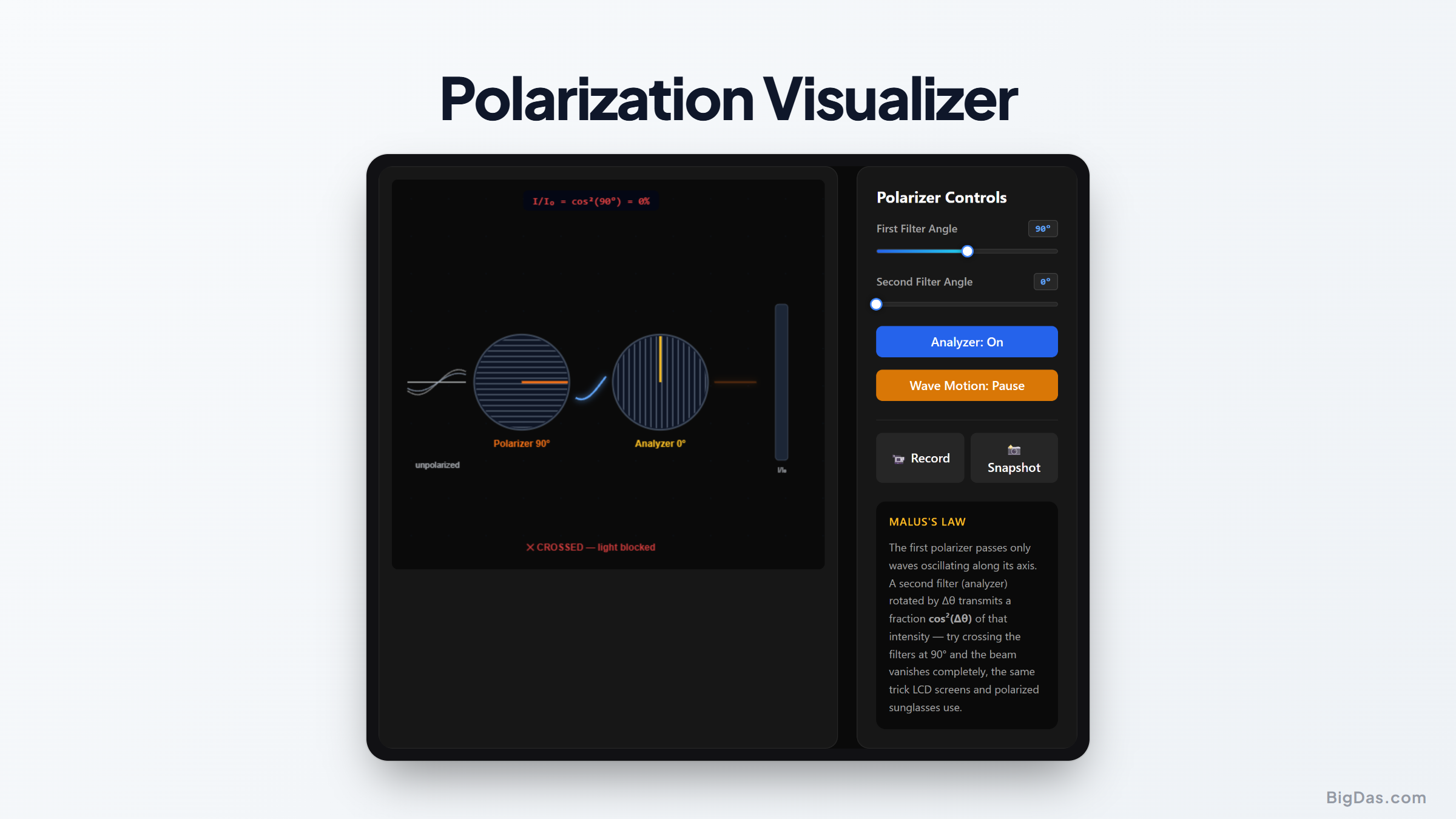
 Generated infographic and interface snapshot for Polarization Visualizer
Interactive Optics Simulation: Understanding Malus Law with the Polarization Visualizer
Light carries information that the human eye cannot see directly. Polarization is one of these hidden properties. Brightness and color are visible, but the orientation of the electric field oscillation is not.
Demonstrating polarization in a classroom or lab requires optical benches, light sources, and physical filters. This equipment is expensive, fragile, and hard for a large group to observe at the same time.
The Polarization Visualizer solves this problem. It is a free browser-based simulation that models how light waves interact with two polarizing filters. Users can rotate the filters and watch the transmitted intensity follow Malus law in real time.
What is Polarization Visualizer?
The Polarization Visualizer is an educational simulation that models electromagnetic wave behavior through polarizing filters.
Light is a transverse wave, so its electric and magnetic fields oscillate perpendicular to the direction of travel. Unpolarized light, such as sunlight or incandescent bulb light, contains oscillations in all directions perpendicular to the beam.
A polarizer is a filter that transmits only the component of the electric field aligned with its transmission axis. Unpolarized light entering a polarizer emerges as linearly polarized light.
The simulation places two polarizers in the path of a light beam. The first polarizes the light, and the second (the analyzer) controls how much of that polarized light reaches the observer. Rotating the analyzer changes the transmitted intensity according to Malus law:
$$I = I_0 \cos^2(\theta)$$
where $I$ is the transmitted intensity, $I_0$ is the intensity entering the analyzer, and $\theta$ is the angle between the transmission axes of the two polarizers.
Key Features
Interactive Axis Control
Both polarizers can be rotated to any angle. The transmitted wave updates immediately, which makes the angle-intensity relationship intuitive rather than memorized.
Visual Wave Representation
The simulation shows the electric field vector, not just a dimmer light source. The wave amplitude visibly shrinks as the angle between the polarizers increases, making wave projection concrete.
Graphical Output
The intensity curve is plotted alongside the wave model. Watching the amplitude drop while the curve follows $\cos^2(\theta)$ connects the math to the physics.
No Equipment Required
A real optics lab needs a bench, light source, polarizers, and a sensor. The simulation replaces all of that with a browser tab.
Cross-Platform
It runs in any modern browser on tablets, laptops, and smartphones. No download or installation is needed.
How to Use It
Open the simulation. You will see a light wave traveling from left to right through two polarizers.
Observe the incoming wave. Before the first filter, oscillations appear in multiple planes, representing unpolarized light.
Pass through the first polarizer. The wave becomes confined to a single plane. It is now linearly polarized.
Find the analyzer control. The second polarizer is the analyzer. Rotate it by dragging the handle or entering a degree value.
Rotate from 0° to 90°. At 0° the axes are aligned and intensity is maximum. Near 45° the amplitude starts to drop.
Stop at 90°. This is the crossed-polarizer configuration. The amplitude reaches zero, because $\cos(90°) = 0$.
Continue to 180°. The amplitude grows again and reaches its second maximum when the axes realign.
Use Cases
For Physics Educators
Drawing 3D waves on a whiteboard is difficult and often confusing. The simulation can be projected during a lecture to show polarization dynamics clearly.
For Students
If the intensity drop during filter rotation is not obvious from a textbook, a few minutes of interaction usually makes the concept click.
For Lab Preparation
Students can use the simulation as a pre-lab activity. Familiarity with the theory before handling physical polarizers reduces equipment damage and improves lab time.
For Photographers and Tech Enthusiasts
Photographers use polarizing filters to cut glare and darken skies. LCDs use crossed polarizers to control pixel brightness. Malus law is the underlying principle in both cases.
FAQ
What is the difference between polarization and intensity?
Polarization is the orientation of the electric field oscillation. Intensity is the energy carried by the wave. A polarizer changes polarization and reduces intensity because it blocks components not aligned with its axis.
Why does Malus law use a squared cosine term?
The polarizer transmits the component of the electric field parallel to its axis, which is proportional to $\cos(\theta)$. Since intensity is proportional to the square of the electric field amplitude, the transmitted intensity is proportional to $\cos^2(\theta)$.
What happens if a third polarizer is inserted between two crossed polarizers?
With two polarizers at 90°, no light passes through. Adding a third polarizer at 45° between them allows light to pass, because the middle polarizer rotates the polarization state so that a component aligns with the final analyzer.
Is this simulation free to use?
Yes. The Polarization Visualizer is free, requires no registration, and has no subscription fees.
Summary
The Polarization Visualizer turns a 3D wave concept into a direct interactive experience. Plotting the wave vector alongside the $\cos^2(\theta)$ intensity curve links the equation to the physical model. It is a practical resource for lesson planning, exam study, or general curiosity about wave optics.